Flexible rule inference and stabile rule representations from task context prediciton.
Introduction
Humans flexibly adapt their behavior to changes in the environment. In the Wisconsin Card Sorting Test (WCST; Grant & Berg, 1948), for example, participants have to infer which hidden rule currently determines the correct response, and adapt their strategy when the rule switches unannounced.
The Wisconsin Neural Network (WiNN; Sommers et al., 2025) solves an image-based version of this task by inferring a context state that signals which rule is active. At every rule switch, however, it searches for a new context state, even for rules it has solved many times before. Natural environments instead carry temporal regularities that memory could exploit to facilitate rule inference.
We therefore extend WiNN with a sequence memory, RNN-FW, that learns the order of rules and predicts the context state for the upcoming rule. We ask two questions: Does sequence memory speed up adaptation when rules follow a predictable order? And can rule switches be detected from WiNN's loss alone, without being told when they happen?
Methods
WiNN
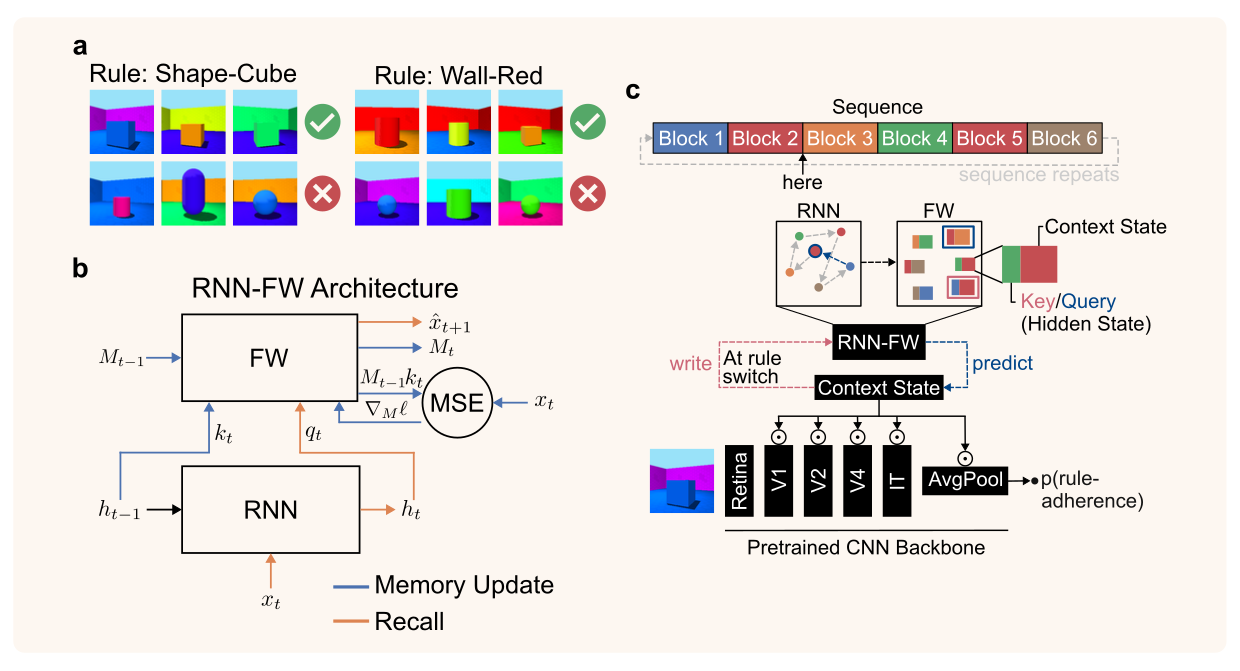
The Wisconsin Neural Network (WiNN; Sommers et al., 2025) flexibly adapts its stimulus-response mappings when a rule changes. It processes one image at a time and has to decide whether the image follows the currently active rule. The images come from the 3D Shapes dataset (Kim and Mnih, 2018) and show an object in front of a wall and on a floor. Object, wall and floor can each take one of ten colors, and the object one of four shapes. A rule refers to a single value of one of these factors, such as "the shape is cube" and "the wall is red" (Figure 1a). Selecting three values per factor results in 12 rules. Each rule is active for a block of 800 images, half of which follow the rule, and then switches without warning. An experiment consists of ten sequences of these 12 blocks, with the block order randomly shuffled in each sequence.
Because the same image has to be mapped differently depending on the active rule, a standard CNN would have to update its weights at every rule switch and would overwrite previously learned mappings.
WiNN avoids this catastrophic forgetting by separating stable features from flexible modulation. Its CNN backbone is pretrained on MiniEcoset (Thorat et al., 2023) and frozen. A context state $c$ modulates the activations of each CNN layer $l$ multiplicatively through attention weights:
$$x^l = \text{ReLU}\left(\text{LN}^l\left(W^l_\text{CNN} x^{l-1}\right)\right) \odot \left(1 + W^l_\text{attn} c\right),$$
where $\text{LN}$ is layer normalization. A modulation term above 1 amplifies a unit's activity, and a term below 1 suppresses it. With $c=0$, the network runs unmodulated. A linear readout then predicts from the last layer whether the image follows the rule.
WiNN is trained with a fast-and-slow learning routine. When WiNN misclassifies an image, its context state $c$ is updated by gradient descent (learning rate 0.01) until the image is classified correctly, for at most 100 steps. Afterwards, the attention and readout weights take a single gradient step (learning rate 0.0001), regardless of whether the classification was correct.
The context state is fast and can quickly move to a representation that decreases the loss. The attention and readout weights are slow and gradually encode the rule mappings. Because the context state quickly decrease the error after a rule switch, the slow weights receive only small updates, and previously learned mappings are preserved. Once the mappings are learned, WiNN only has to find the context state that activates the mapping of the incoming rule.
However, this search starts from the previous block's context state at every rule switch, and it is repeated each time a rule returns, even for rules WiNN has solved many times before. In the original setup, the block order is shuffled in every sequence, so the next rule cannot be predicted. In many real-world settings, however, tasks follow a predictable order. We therefore present the blocks in a fixed order that repeats across sequences, and extend WiNN with a sequence memory that learns this order. At each rule switch, context inference can then start from a well-informed context state.
WiNN + RNN-FW
To learn this order, we build an RNN with an external fast-weight memory (RNN-FW; Figure 1b). The RNN tracks the position in the sequence, while the fast-weight memory $\mathbf{M}$ stores what comes next. The slow weights, meaning all projections, the RNN weights and two scalars $\eta$ and $\alpha$, are trained beforehand on repeating sequences of random vectors and then kept fixed. The fast weights, in contrast, change at every step, so the model can memorize a new sequence on the fly.
Let $t$ count the rule switches. At the switch after block $t$, WiNN has just inferred the context state $\mathbf{c}_t$, and RNN-FW performs three operations.
1. Write. The memory stores the association between the previous hidden state and the new context state. Both are projected into a common space, and the key is L2-normalized:
$$ \mathbf{k}_t = \frac{\mathbf{W}^K\mathbf{h}_{t-1}}{\lVert \mathbf{W}^K\mathbf{h}_{t-1}\rVert_2}, \qquad \mathbf{v}_t = \mathbf{W}^V\mathbf{c}_t $$
The memory then takes one gradient step on the error between what it currently associates with the key and the new value, $\tfrac{1}{2}\lVert\mathbf{M}_{t-1}\mathbf{k}_t - \mathbf{v}_t\rVert_2^2$, combined with a multiplicative decay:
$$ \mathbf{M}_t = (1-\alpha)\,\mathbf{M}_{t-1} - \eta\,(\mathbf{M}_{t-1}\mathbf{k}_t - \mathbf{v}_t)\,\mathbf{k}_t^\top $$
This is the delta rule (Widrow and Hoff, 1960) with decay, similar to Gated DeltaNet (Yang et al., 2025), with learning rate $\eta$ and forget gate $\alpha$.
2. Integrate. The RNN receives the context state as input and updates its hidden state:
$$ \mathbf{h}_t = \tanh\big(\mathbf{W}_{ih}\,\mathbf{c}_t + \mathbf{W}_{hh}\,\mathbf{h}_{t-1} + \mathbf{b}\big) $$
3. Read. A query built from the updated hidden state retrieves the prediction for the next block, which is projected back into context state space:
$$ \mathbf{q}_t = \frac{\mathbf{W}^Q\mathbf{h}_t}{\lVert\mathbf{W}^Q\mathbf{h}_t\rVert_2}, \qquad \hat{\mathbf{c}}_{t+1} = \mathbf{W}^O\,\mathbf{M}_t\,\mathbf{q}_t $$
WiNN starts the next block from $\hat{\mathbf{c}}_{t+1}$ and refines it with its usual learning routine, and the refined state is written into memory at the next switch (Figure 1c). Because keys and queries come from the hidden state, which carries the sequence history, the same rule can be followed by different rules at different positions in the sequence.
Detecting rule switches. These operations require knowing when the rule switches. WiNN + RNN-FW is given the true switch times, while WiNN + RNN-FW-Detect infers them from WiNN's loss, which is low at the end of a block and jumps when the old context state stops working. For each image $n$, it tracks moving averages of the loss $\ell_n$ (measured before any updates) and of its absolute deviation:
$$ \mu_n = (1-\rho)\,\mu_{n-1} + \rho\,\ell_n, \qquad d_n = (1-\rho)\,d_{n-1} + \rho\,\lvert\ell_n - \mu_{n-1}\rvert $$
A rule switch is detected when the loss is surprisingly high relative to these averages, i.e. when
$$ z_n = \frac{\ell_n - \mu_{n-1}}{\sqrt{d_{n-1}} + \epsilon} $$
exceeds a threshold found by hyperparameter optimization.
Results
RNN-FW
Before looking at how RNN-FW accelerates WiNN's rule inference, we test it on its own. We train it on repeating sequences of random vectors and compare it with two parameter-matched models: a standard RNN without external memory, and a feedforward fast-weight model (FF-FW), which has no recurrent state and accesses the memory based only on the current sequence element.
We test sequences of length 10 and 30. In non-ambiguous sequences, every element has exactly one successor. In ambiguous sequences, at least one element is followed by two different successors, as in A → B → A → C.
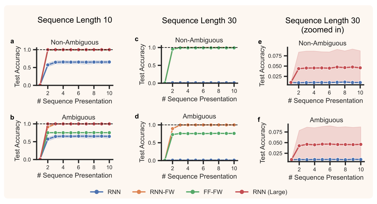
On non-ambiguous sequences, RNN-FW and FF-FW predict the sequence correctly after seeing it only once (Figure 2). The RNN performs much worse at length 10 and fails completely at length 30. On ambiguous sequences, RNN-FW reaches perfect accuracy from the third presentation onward, while FF-FW's accuracy drops. Without a hidden state, both occurrences of A produce the same key, so FF-FW cannot associate them with different successors. The RNN performs as poorly as before.
Even an RNN with 1024 instead of 220 hidden units predicts sequences of length 10 but still fails at length 30. This is because the RNN has to store both the sequence elements and their order in its hidden state, whereas RNN-FW offloads the elements to the fast weights and only has to track the position in the sequence.
WiNN + RNN-FW
We evaluate the models in two settings. In the pretrained setting, WiNN has learned the 12 rules before the experiment, so its attention and readout weights are already adapted to them. In the untrained setting, these weights are randomly initialized at the start of the experiment.
WiNN's loss reliably signals rule switches
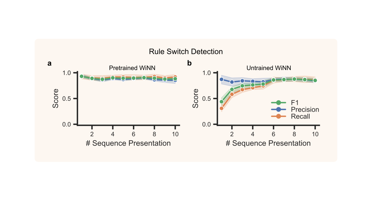
For a pretrained WiNN, the detector reaches a precision and recall of about 0.9 across all sequence presentations (Figure 3), so the loss reliably signals when the rule switches. For an untrained WiNN, recall is low at first. WiNN has not learned the rules yet, and its high loss hides the jump at a switch. As WiNN learns to classify the images, the loss within blocks decreases and recall catches up after about six presentations. Precision stays high throughout, because rule switches always cause large loss increases, while false detections within a block remain rare.
RNN-FW accelerates rule inference
To test whether RNN-FW accelerates WiNN on sequences with a fixed block order, we measure two things: the number of context state updates per sequence, and the number of images WiNN needs to reach a criterion of 90% accuracy over ten consecutive images. We focus on the pretrained WiNN. An untrained WiNN first has to learn the rules, so all models need many updates at the beginning, but afterwards the same pattern emerges.
We also compare against a control, WiNN (Context Reset), that sets the context state to the zero vector at every rule switch. Standard WiNN always starts its search from the previous rule's context state, which may be far from a good state for the new rule. The reset control tests whether a fresh starting point alone already helps, without any memory.
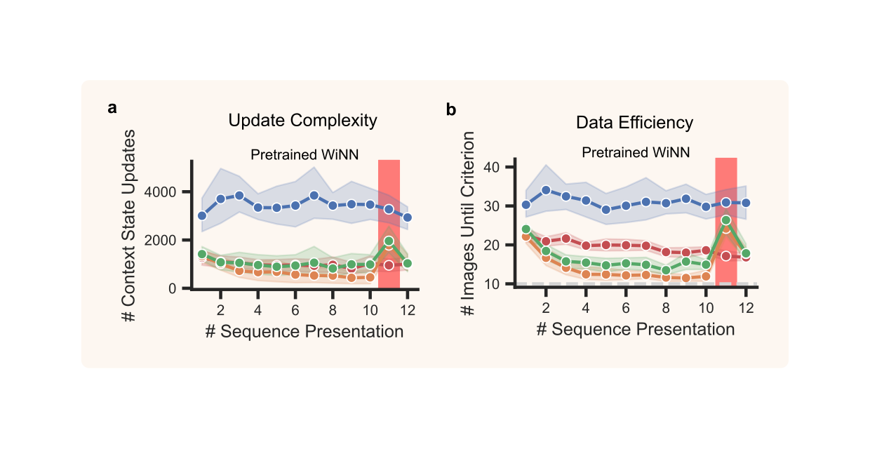
Standard WiNN performs the most context state updates (Figure 4). WiNN + RNN-FW-Detect and the reset control perform a similar number of updates, and WiNN + RNN-FW performs the fewest. The gap between the two RNN-FW variants shows that loss-based detection is not perfect as missed or false detections can put the RNN out of step with the sequence.
Because the reset control performs as well as WiNN + RNN-FW-Detect, update counts alone cannot tell whether the benefit comes from sequence memory. In fact, already in the first sequence, before the memory has stored anything, the RNN-FW models and the reset control need fewer updates than WiNN. This comes from simply not starting at the previous rule's context state. To test whether the models also use the learned order, the 11th sequence shuffles the block order. WiNN and the reset control are unaffected, while the number of updates rises sharply for both RNN-FW models, because their predictions no longer match the upcoming rules. When the original order returns in the 12th sequence, both recover, though not completely.
The number of images until the criterion is met shows the same picture. Both RNN-FW models need far fewer images than WiNN and also fewer than the reset control. WiNN + RNN-FW even approaches ten images, the minimum needed to evaluate the criterion, meaning it solves the new rule almost immediately after a switch. In the shuffled 11th sequence, the number of images again rises sharply for both RNN-FW variants.
Sequence memory stabilizes context state representations
Sequence memory does not only speed up adaptation, it also changes where the context states end up. When a rule returns, does WiNN find the same context state as before, or a different one each time?
To find out, we take the context state at the end of every block and compute a representational dissimilarity matrix (RDM) for each model and seed. Each entry is the dissimilarity (1 − Pearson correlation) between the context states of two blocks, which gives a 120 × 120 matrix for 10 sequence repetitions × 12 blocks. We compare these RDMs with three hypothesis RDMs (Figure 5):
- Rule: blocks with the same rule have similar context states, regardless of when they occurred.
- Repetition: blocks from the same sequence repetition have similar context states.
- Temporal: context states become less similar the further apart two blocks are in time.
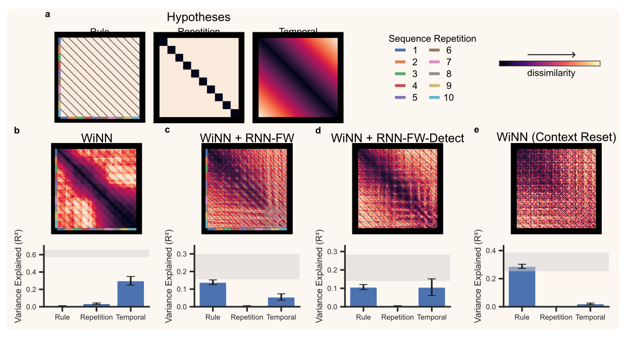
The hypotheses overlap, since blocks from the same repetition are also close in time. We therefore fit a linear regression that predicts each model's RDM from all three hypothesis RDMs at once. The unique variance of a hypothesis is how much the explained variance (R²) drops when that hypothesis is removed from the regression. As a reference, the upper noise ceiling estimates the best R² we can expect, given how much the RDMs vary across seeds.
The standard WiNN's context states are organized by time (Figure 5). The temporal hypothesis explains substantial unique variance, while the rule hypothesis explains almost none. The same rule therefore ends up in a different place in each repetition, as the context states gradually drift over the experiment. Even all three hypotheses together do not reach the noise ceiling, so part of the structure remains unexplained.
With sequence memory, the picture changes. For WiNN + RNN-FW, the rule hypothesis explains the most unique variance, followed by the temporal hypothesis. For WiNN + RNN-FW-Detect, both explain similar amounts, with the temporal hypothesis varying more across seeds, consistent with imperfect switch detection. The reset control is organized almost entirely by rule, reaching the noise ceiling, while the temporal hypothesis explains close to nothing. The repetition hypothesis explains almost no unique variance in any model, likely because blocks from the same repetition are also close in time.
Both memory and a consistent starting point thus pull context inference back to rule-specific regions, reducing the representational drift of the standard WiNN.
Conclusion
Sequence memory turns WiNN's search at every rule switch into an informed prediction. When rules follow a predictable order, RNN-FW supplies context states that reduce the number of context state updates and let WiNN solve a new rule almost immediately after a switch. Once WiNN has learned the rules, its loss reliably signals rule switches, and the detection-based model keeps most of the benefit.
Two design choices make this work. First, the memory is keyed on the position in the sequence rather than on the input. Since the same images appear under every rule, the input cannot tell which context state to retrieve, but the position in the sequence can. Second, the RNN only tracks this position, while the fast weights store the context states, which is much more parameter efficient than storing everything in the hidden state.
The reset control shows that part of the benefit simply comes from not starting at the previous rule's context state. On top of this, sequence memory lets WiNN exploit a predictable order, and like the reset, it organizes context states by rule instead of letting them drift over time. The incomplete recovery after the shuffled sequence also shows a limitation: new memory writes can interfere with a sequence that has already been learned.
Whether this temporal-position memory extends to higher-dimensional task structure, where prediction requires integrating over relational rather than purely sequential structure, remains open.
References
Grant, David A and Esta Berg (1948). “A behavioral analysis of degree of
reinforcement and ease of shifting to new responses in a Weigl-type card-sorting problem.” In: Journal of experimental psychology 38.4, p. 404. ↩
Sommers, R. P., Thorat, S., Anthes, D., & Kietzmann, T. C. (2025). Sparks of cognitive flexibility: self-guided context inference for flexible stimulus-response mapping by attentional routing. arXiv preprint arXiv:2502.15634. ↩a ↩b ↩c
Thorat, Sushrut, Adrien Doerig, and Tim C. Kietzmann (2023). Characterising representation dynamics in recurrent neural networks for object recognition. arXiv: 2308.12435 [cs.CV]. url: https://arxiv.org/abs/2308.12435. ↩
Kim, H. & Mnih, A.. (2018). Disentangling by Factorising. Proceedings of the 35th International Conference on Machine Learning, in Proceedings of Machine Learning Research 80:2649-2658 Available from https://proceedings.mlr.press/v80/kim18b.html. ↩a ↩b
Hoff, M. E., & Widrow, B. (1960, August). Adaptive switching circuits. In 1960 IRE WESCON Convention Recor (pp. 96-104). ↩
Yang, Songlin, Jan Kautz, and Ali Hatamizadeh (2025). “Gated delta networks: Improving mamba2 with delta rule”. In: International Conference on Learning Representations. Vol. 2025, pp. 29687–29707. ↩